Compare Hankel and Fourier Transforms
This will compare the forward and inverse transforms for both Hankel and Fourier by either computing partial derivatives of solving a parital differential equation.
This notebook focuses on the Laplacian operator in the case of radial symmetry.
Consider two 2D circularly-symmetric functions \(f(r)\) and \(g(r)\) that are related by the following differential operator,
compute the Laplacian to obtain \(g(r)\) 2. Given \(g(r)\), invert the Laplacian to obtain \(f(r)\)
We can use the 1D Hankel (or 2D Fourier) transform to compute the Laplacian in three steps: 1. Compute the Forward Transform
This is easily done in two-dimensions using the Fast Fourier Transform (FFT) but one advantage of the Hankel transform is that we only have a one-dimensional transform.
Import Relevant Libraries
In [2]:
# Import Libraries

import numpy as np                                                        # Numpy
from scipy.fftpack import fft2, ifft2, fftfreq, ifftn, fftn               # Fourier
from hankel import HankelTransform, SymmetricFourierTransform             # Hankel
from scipy.interpolate import InterpolatedUnivariateSpline as spline      # Splines
import matplotlib.pyplot as plt                                           # Plotting
import matplotlib as mpl
from os import path
%matplotlib inline
In [34]:
## Put the prefix to the figure directory here for your computer. If you don't want to save files, set to empty string, or None.
prefix =  path.expanduser("~/Documents/Projects/HANKEL/laplacian_paper/Figures/")
Standard Plot Aesthetics
In [4]:
mpl.rcParams['lines.linewidth'] = 2
mpl.rcParams['xtick.labelsize'] = 13
mpl.rcParams['ytick.labelsize'] = 13
mpl.rcParams['font.size'] = 15
mpl.rcParams['axes.titlesize'] = 14
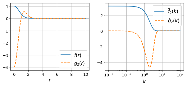
Define Sample Functions
We define the two functions
In [5]:
# Define Gaussian

f = lambda r: np.exp(-r**2)

# Define Laplacian Gaussian function

g = lambda r: 4.0*np.exp(-r**2)*(r**2 - 1.0)
We can also define the FTs of these functions analytically, so we can compare our numerical results:
In [6]:
fhat = lambda x : np.pi*np.exp(-x**2/4.)
ghat = lambda x : -x**2*fhat(x)
In [7]:
# Make a plot of the sample functions

fig, ax = plt.subplots(1,2,figsize=(10,4))
r = np.linspace(0,10,128)
ax[0].plot(r, f(r), label=r"$f(r)$")
ax[0].plot(r, g(r), label=r'$g_2(r)$', ls="--")
ax[0].legend()
ax[0].set_xlabel(r"$r$")
ax[0].grid(True)

k = np.logspace(-2,2,128)
ax[1].plot(k, fhat(k), label=r"$\hat{f}_2(k)$")
ax[1].plot(k, ghat(k), label=r'$\hat{g}_2(k)$', ls="--")
ax[1].legend()
ax[1].set_xlabel(r"$k$")
ax[1].grid(True)
ax[1].set_xscale('log')
#plt.suptitle("Plot of Sample Functions")


if prefix:
    plt.savefig(path.join(prefix,"sample_function.pdf"))
Define Transformation Functions
In [8]:
def ft_transformation_2d(f,x, inverse=False):

    xx,yy = np.meshgrid(x,x)
    r = np.sqrt(xx**2 + yy**2)

    # Appropriate k-space values
    k = 2*np.pi*fftfreq(len(x),d=x[1]-x[0])
    kx,ky = np.meshgrid(k,k)
    K2 = kx**2+ky**2

    # The transformation
    if not inverse:
        g2d = ifft2(-K2 * fft2(f(r)).real).real
    else:
        invK2 = 1./K2
        invK2[np.isinf(invK2)] = 0.0

        g2d = ifft2(-invK2 * fft2(f(r)).real).real

    return x[len(x)//2:], g2d[len(x)//2,len(x)//2:]
In [27]:
def ht_transformation_nd(f,N_forward,h_forward,K,r,ndim=2, inverse=False, N_back=None, h_back=None,
                         ret_everything=False):

    if N_back is None:
        N_back = N_forward
    if h_back is None:
        h_back = h_forward

    # Get transform of f
    ht = SymmetricFourierTransform(ndim=ndim, N=N_forward, h=h_forward)

    if ret_everything:
        fhat, fhat_cumsum = ht.transform(f, K, ret_cumsum=True, ret_err=False)
    else:
        fhat = ht.transform(f, K, ret_err = False)

    # Spectral derivative
    if not inverse:
        ghat = -K**2 * fhat
    else:
        ghat = -1./K**2 * fhat

    # Transform back to physical space via spline
    # The following should give best resulting splines for most kinds of functions
    # Use log-space y if ghat is either all negative or all positive, otherwise linear-space
    # Use order 1 because if we have to extrapolate, this is more stable.
    # This will not be a good approximation for discontinuous functions... but they shouldn't arise.
    if np.all(ghat<=1e-13):
        g_ = spline(K[ghat<0],np.log(-ghat[ghat<0]),k=1)
        ghat_spline = lambda x : -np.exp(g_(x))
    elif np.all(ghat>=-1e-13):
        g_ = spline(K[ghat>0],np.log(ghat[ghat>0]),k=1)
        ghat_spline = lambda x : np.exp(g_(x))
    else:
        g_ = spline(K,ghat,k=1)
        ghat_spline = g_

    if N_back != N_forward or h_back != h_forward:
        ht2 = SymmetricFourierTransform(ndim=ndim, N=N_back, h=h_back)
    else:
        ht2 = ht

    if ret_everything:
        g, g_cumsum = ht2.transform(ghat_spline, r, ret_err=False, inverse=True, ret_cumsum=True)
    else:
        g = ht2.transform(ghat_spline, r, ret_err=False, inverse=True)

    if ret_everything:
        return g, g_cumsum, fhat,fhat_cumsum, ghat, ht,ht2, ghat_spline
    else:
        return g
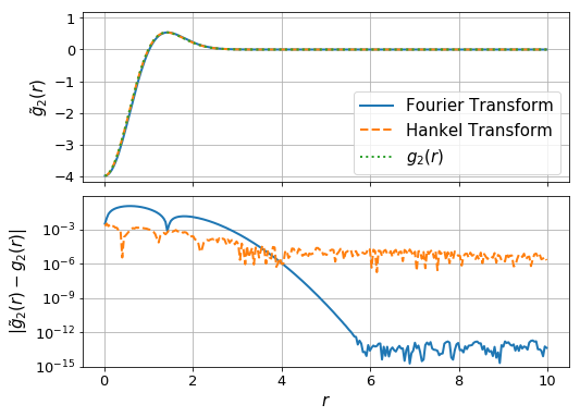
Forward Laplacian
We can simply use the defined functions to determine the foward laplacian in each case. We just need to specify the grid.
In [49]:
L = 10.
N = 256
dr = L/N

x_ft = np.linspace(-L+dr/2,L-dr/2,2*N)
r_ht = np.linspace(dr/2,L-dr/2,N)
We also need to choose appropriate parameters for the forwards/backwards
Hankel Transforms. To do this, we can use the get_h function in the
hankel library:
In [50]:
from hankel import get_h

hback, res, Nback = get_h(ghat, nu=2, K=r_ht[::10], cls=SymmetricFourierTransform, atol=1e-8, rtol=1e-4, inverse=True)
K = np.logspace(-2, 2, N) # These values come from inspection of the plot above, which shows that ghat is ~zero outside these bounds
hforward, res, Nforward = get_h(f, nu=2, K=K[::50], cls=SymmetricFourierTransform, atol=1e-8, rtol=1e-4)
hforward, Nforward, hback, Nback
Out[50]:
(9.765625e-05, 2207, 0.000390625, 534)
In [51]:
## FT
r_ft, g_ft = ft_transformation_2d(f,x_ft)

# Note: r_ft is equivalent to r_ht

## HT
g_ht = ht_transformation_nd(f,N_forward=Nforward, h_forward=hforward, N_back=Nback, h_back=hback, K = K, r = r_ht)
Now we plot the calculated functions against the analytic result:
In [52]:
fig, ax = plt.subplots(2,1, sharex=True,gridspec_kw={"hspace":0.08},figsize=(8,6))

ax[0].plot(r_ft,g_ft, label="Fourier Transform", lw=2)
ax[0].plot(r_ht, g_ht, label="Hankel Transform", lw=2, ls='--')
ax[0].plot(r_ht, g(r_ht), label = "$g_2(r)$", lw=2, ls = ':')
ax[0].legend(fontsize=15)

#ax[0].xaxis.set_ticks([])
ax[0].grid(True)
ax[0].set_ylabel(r"$\tilde{g}_2(r)$",fontsize=15)
ax[0].set_ylim(-4.2,1.2)

ax[1].plot(r_ft, np.abs(g_ft-g(r_ft)), lw=2)
ax[1].plot(r_ht, np.abs(g_ht-g(r_ht)),lw=2, ls='--')
#ax[1].set_ylim(-1,1)
ax[1].set_yscale('log')
#ax[1].set_yscale("symlog",linthreshy=1e-6)
ax[1].set_ylabel(r"$|\tilde{g}_2(r)-g_2(r)|$",fontsize=15)
ax[1].set_xlabel(r"$r$",fontsize=15)
ax[1].set_ylim(1e-15, 0.8)
plt.grid(True)

if prefix:
    fig.savefig(path.join(prefix,"forward_laplacian.pdf"))
Timing for each calculation:
In [53]:
%timeit ft_transformation_2d(f,x_ft)
%timeit ht_transformation_nd(f,N_forward=Nforward, h_forward=hforward, N_back=Nback, h_back=hback, K = K, r = r_ht)
10 loops, best of 3: 17 ms per loop
100 loops, best of 3: 19.7 ms per loop
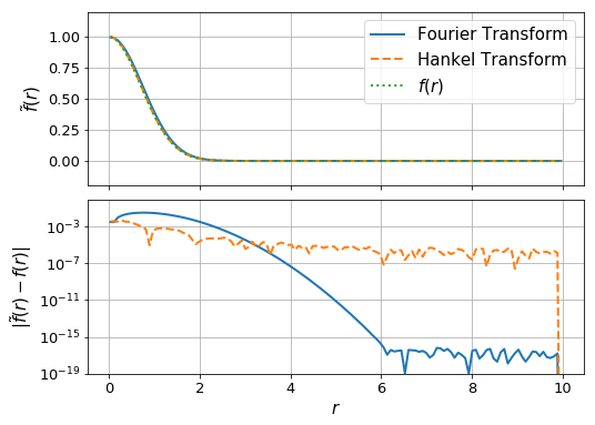
Inverse Laplacian
We use the 1D Hankel (or 2D Fourier) transform to compute the Laplacian in three steps: 1. Compute the Forward Transform
Again, we compute the relevant Hankel parameters:
In [35]:
hback, res, Nback = get_h(fhat, nu=2, K=r_ht[::10], cls=SymmetricFourierTransform, atol=1e-8, rtol=1e-4, inverse=True)
K = np.logspace(-2, 2, N) # These values come from inspection of the plot above, which shows that ghat is ~zero outside these bounds
hforward, res, Nforward = get_h(g, nu=2, K=K[::50], cls=SymmetricFourierTransform, atol=1e-8, rtol=1e-4)
hforward,Nforward,hback,Nback
Out[35]:
(4.8828125e-05, 1266, 0.00078125, 375)
In [36]:
## FT
r_ft, f_ft = ft_transformation_2d(g,x_ft, inverse=True)

# Note: r_ft is equivalent to r_ht

## HT
f_ht = ht_transformation_nd(g,N_forward=Nforward, h_forward=hforward,N_back=Nback, h_back=hback, K = K, r = r_ht, inverse=True)
/home/steven/miniconda3/envs/hankel2/lib/python2.7/site-packages/ipykernel/__main__.py:15: RuntimeWarning: divide by zero encountered in divide
In [37]:
fig, ax = plt.subplots(2,1, sharex=True,gridspec_kw={"hspace":0.08},figsize=(8,6))
#np.mean(f(r_ft)) - np.mean(f_ft)
ax[0].plot(r_ft,f_ft + f(r_ft)[-1] - f_ft[-1], label="Fourier Transform", lw=2)
ax[0].plot(r_ht, f_ht, label="Hankel Transform", lw=2, ls='--')
ax[0].plot(r_ht, f(r_ht), label = "$f(r)$", lw=2, ls = ':')
ax[0].legend()

ax[0].grid(True)
ax[0].set_ylabel(r"$\tilde{f}(r)$",fontsize=15)
ax[0].set_ylim(-0.2,1.2)
#ax[0].set_yscale('log')

ax[1].plot(r_ft, np.abs(f_ft + f(r_ft)[-1] - f_ft[-1] -f(r_ft)), lw=2)
ax[1].plot(r_ht, np.abs(f_ht -f(r_ht)),lw=2, ls='--')

ax[1].set_yscale('log')
ax[1].set_ylabel(r"$|\tilde{f}(r)-f(r)|$",fontsize=15)
ax[1].set_xlabel(r"$r$",fontsize=15)
ax[1].set_ylim(1e-19, 0.8)
plt.grid(True)

if prefix:
    fig.savefig(path.join(prefix,"inverse_laplacian.pdf"))
In [28]:
%timeit ft_transformation_2d(g,x_ft, inverse=True)
%timeit ht_transformation_nd(g,N_forward=Nforward, h_forward=hforward,N_back=Nback, h_back=hback, K = K, r = r_ht, inverse=True)
/home/steven/miniconda3/envs/hankel2/lib/python2.7/site-packages/ipykernel/__main__.py:15: RuntimeWarning: divide by zero encountered in divide
10 loops, best of 3: 19.3 ms per loop
10 loops, best of 3: 30.6 ms per loop
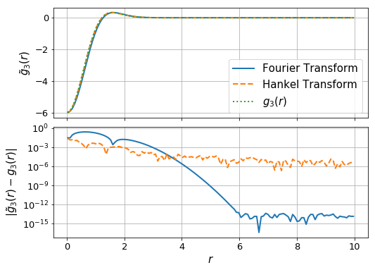
3D Problem (Forward)
We need to define the FT function again, for 3D:
In [38]:
def ft_transformation_3d(f,x, inverse=False):

    r = np.sqrt(np.sum(np.array(np.meshgrid(*([x]*3)))**2,axis=0))

    # Appropriate k-space values
    k = 2*np.pi*fftfreq(len(x),d=x[1]-x[0])
    K2 = np.sum(np.array(np.meshgrid(*([k]*3)))**2,axis=0)

    # The transformation
    if not inverse:
        g2d = ifftn(-K2 * fftn(f(r)).real).real
    else:
        invK2 = 1./K2
        invK2[np.isinf(invK2)] = 0.0

        g2d = ifftn(-invK2 * fftn(f(r)).real).real

    return x[len(x)/2:], g2d[len(x)/2,len(x)/2, len(x)/2:]
We also need to define the 3D laplacian function:
In [39]:
g3 = lambda r: 4.0*np.exp(-r**2)*(r**2 - 1.5)
fhat_3d = lambda x : np.pi**(3./2)*np.exp(-x**2/4.)
ghat_3d = lambda x : -x**2*fhat_3d(x)
In [40]:
L = 10.
N = 128
dr = L/N

x_ft = np.linspace(-L+dr/2,L-dr/2,2*N)
r_ht = np.linspace(dr/2,L-dr/2,N)
Again, choose our resolution parameters
In [32]:
hback, res, Nback = get_h(ghat_3d, nu=3, K=r_ht[::10], cls=SymmetricFourierTransform, atol=1e-8, rtol=1e-4, inverse=True)
K = np.logspace(-2, 2, 2*N) # These values come from inspection of the plot above, which shows that ghat is ~zero outside these bounds
hforward, res, Nforward = get_h(f, nu=3, K=K[::50], cls=SymmetricFourierTransform, atol=1e-8, rtol=1e-4)
hforward, Nforward, hback, Nback
Out[32]:
(9.765625e-05, 2207, 0.00078125, 375)
In [33]:
## FT
r_ft, g_ft = ft_transformation_3d(f,x_ft)

# Note: r_ft is equivalent to r_ht

## HT
K = np.logspace(-1.0,2.,N)
g_ht = ht_transformation_nd(f,N_forward=Nforward, h_forward=hforward, N_back=Nback, h_back=hback, K = K, r = r_ht, ndim=3)
In [65]:
fig, ax = plt.subplots(2,1, sharex=True,gridspec_kw={"hspace":0.08},figsize=(8,6))

ax[0].plot(r_ft,g_ft, label="Fourier Transform", lw=2)
ax[0].plot(r_ht, g_ht, label="Hankel Transform", lw=2, ls='--')
ax[0].plot(r_ht, g3(r_ht), label = "$g_3(r)$", lw=2, ls = ':')
ax[0].legend(fontsize=15)

#ax[0].xaxis.set_ticks([])
ax[0].grid(True)
ax[0].set_ylabel(r"$\tilde{g}_3(r)$",fontsize=15)
#ax[0].set_ylim(-4.2,1.2)

ax[1].plot(r_ft, np.abs(g_ft-g3(r_ft)), lw=2)
ax[1].plot(r_ht, np.abs(g_ht-g3(r_ht)),lw=2, ls='--')

ax[1].set_yscale('log')
ax[1].set_ylabel(r"$|\tilde{g}_3(r)-g_3(r)|$",fontsize=15)
ax[1].set_xlabel(r"$r$",fontsize=15)
plt.grid(True)

if prefix:
    fig.savefig(path.join(prefix,"forward_laplacian_3D.pdf"))
In [72]:
%timeit ht_transformation_nd(f,N_forward=Nforward, h_forward=hforward, N_back=Nback, h_back=hback, K = K, r = r_ht, ndim=3)

%timeit ft_transformation_3d(f,x_ft)
100 loops, best of 3: 16.3 ms per loop
1 loop, best of 3: 2.66 s per loop
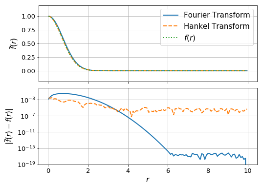
3D Problem (Inverse)
In [41]:
hback, res, Nback = get_h(fhat_3d, nu=3, K=r_ht[::10], cls=SymmetricFourierTransform, atol=1e-8, rtol=1e-4, inverse=True)
K = np.logspace(-2, 2, N) # These values come from inspection of the plot above, which shows that ghat is ~zero outside these bounds
hforward, res, Nforward = get_h(g3, nu=3, K=K[::50], cls=SymmetricFourierTransform, atol=1e-8, rtol=1e-4)
hforward,Nforward,hback,Nback
Out[41]:
(6.103515625e-06, 3576, 0.00078125, 375)
In [46]:
## FT
r_ft, f_ft = ft_transformation_3d(g3,x_ft, inverse=True)

# Note: r_ft is equivalent to r_ht

## HT
f_ht = ht_transformation_nd(g3,ndim=3, N_forward=Nforward, h_forward=hforward,N_back=Nback, h_back=hback, K = K, r = r_ht, inverse=True)
/home/steven/miniconda3/envs/hankel2/lib/python2.7/site-packages/ipykernel/__main__.py:13: RuntimeWarning: divide by zero encountered in divide
In [48]:
fig, ax = plt.subplots(2,1, sharex=True,gridspec_kw={"hspace":0.08},figsize=(8,6))
#np.mean(f(r_ft)) - np.mean(f_ft)
ax[0].plot(r_ft, f_ft + f(r_ft)[-1] - f_ft[-1], label="Fourier Transform", lw=2)
ax[0].plot(r_ht, f_ht + f(r_ft)[-1] - f_ht[-1], label="Hankel Transform", lw=2, ls='--')
ax[0].plot(r_ht, f(r_ht), label = "$f(r)$", lw=2, ls = ':')
ax[0].legend()

ax[0].grid(True)
ax[0].set_ylabel(r"$\tilde{f}(r)$",fontsize=15)
ax[0].set_ylim(-0.2,1.2)
#ax[0].set_yscale('log')

ax[1].plot(r_ft, np.abs(f_ft + f(r_ft)[-1] - f_ft[-1] -f(r_ft)), lw=2)
ax[1].plot(r_ht, np.abs(f_ht + f(r_ft)[-1] - f_ht[-1] -f(r_ht)),lw=2, ls='--')

ax[1].set_yscale('log')
ax[1].set_ylabel(r"$|\tilde{f}(r)-f(r)|$",fontsize=15)
ax[1].set_xlabel(r"$r$",fontsize=15)
ax[1].set_ylim(1e-19, 0.8)
plt.grid(True)

if prefix:
    fig.savefig(path.join(prefix,"inverse_laplacian_3d.pdf"))