Getting Started with Hankel

Usage and Description

Setup

This implementation is set up to allow efficient calculation of multiple functions \(f(x)\). To do this, the format is class-based, with the main object taking as arguments the order of the Bessel function, and the number and size of the integration steps (see Limitations for discussion about how to choose these key parameters).

For any general integration or transform of a function, we perform the following setup:

import hankel
from hankel import HankelTransform     # Import the basic class
print("Using hankel v{}".format(hankel.__version__))

Using hankel v0.3.7

ht = HankelTransform(
    nu= 0,     # The order of the bessel function
    N = 120,   # Number of steps in the integration
    h = 0.03   # Proxy for "size" of steps in integration
)

Alternatively, each of the parameters has defaults, so you needn’t pass any. The order of the bessel function will be defined by the problem at hand, while the other arguments typically require some exploration to set them optimally.

Integration

A Hankel-type integral is the integral

\[\int_0^\infty f(x) J_\nu(x) dx.\]

Having set up our transform with nu = 0, we may wish to perform this integral for \(f(x) = 1\). To do this, we do the following:

# Create a function which is identically 1.
f = lambda x : 1
ht.integrate(f)

(1.0000000000003486, -9.838142836853752e-15)

The correct answer is 1, so we have done quite well. The second element of the returned result is an estimate of the error (it is the last term in the summation). The error estimate can be omitted using the argument ret_err=False.

We may now wish to integrate a different function, say \(x/(x^2 + 1)\). We can do this directly with the same object, without re-instantiating (avoiding unnecessary recalculation):

f = lambda x : x/(x**2 + 1)
ht.integrate(f)

(0.42098875721567186, -2.6150757700135774e-17)

The analytic answer here is \(K_0(1) = 0.4210\). The accuracy could be increased by creating ht with a higher number of steps N, and lower stepsize h (see Limitations).

Transforms

The Hankel transform is defined as

\[F_\nu(k) = \int_0^\infty f(r) J_\nu(kr) r dr.\]

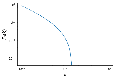
We see that the Hankel-type integral is the Hankel transform of \(f(r)/r\) with \(k=1\). To perform this more general transform, we must supply the \(k\) values. Again, let’s use our previous function, \(x/(x^2 + 1)\).

First we’ll import some libraries to help us visualise:

import numpy as np              # Import numpy
import matplotlib.pyplot as plt
%matplotlib inline

Now do the transform,

k = np.logspace(-1,1,50)             # Create a log-spaced array of k from 0.1 to 10.
Fk = ht.transform(f,k,ret_err=False) # Return the transform of f at k.

and finally plot it:

plt.plot(k,Fk)
plt.xscale('log')
plt.yscale('log')
plt.ylabel(r"$F_0(k)$", fontsize=15)
plt.xlabel(r"$k$", fontsize=15)
plt.show()

Fourier Transforms

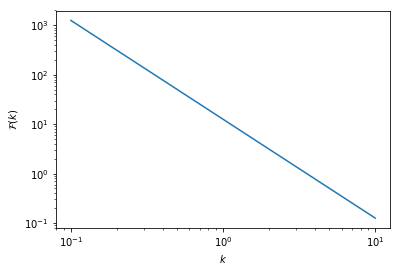
One of the most common applications of the Hankel transform is to solve the radially symmetric n-dimensional Fourier transform:

\[F(k) = \frac{(2\pi)^{n/2}}{k^{n/2-1}} \int_0^\infty r^{n/2-1} f(r) J_{n/2-1}(kr)r dr.\]

We provide a specific class to do this transform, which takes into account the various normalisations and substitutions required, and also provides the inverse transform. The procedure is similar to the basic HankelTransform, but we provide the number of dimensions, rather than the Bessel order directly.

Say we wish to find the Fourier transform of \(f(r) = 1/r\) in 3 dimensions:

# Import the Symmetric Fourier Transform class
from hankel import SymmetricFourierTransform

# Create our transform object, similar to HankelTransform,
# but with ndim specified instead of nu.
ft = SymmetricFourierTransform(ndim=3, N = 200, h = 0.03)

# Create our kernel function to be transformed.
f = lambda r : 1./r

# Perform the transform
Fk = ft.transform(f,k, ret_err=False)

plt.plot(k,Fk)
plt.xscale('log')
plt.yscale('log')
plt.ylabel(r"$\mathcal{F}(k)$")
plt.xlabel(r"$k$")
plt.show()

To do the inverse transformation (which is different by a normalisation constant), merely supply inverse=True to the .transform() method.

Limitations

Efficiency

An implementation-specific limitation is that the method is not perfectly efficient in all cases. Care has been taken to make it efficient in the general sense. However, for specific orders and functions, simplifications may be made which reduce the number of trigonometric functions evaluated. For instance, for a zeroth-order spherical transform, the weights are analytically always identically 1.

Lower-Bound Convergence

Theoretically, since Bessel functions have asymptotic power-law slope of \(n/2 -1\) as \(r \rightarrow 0\), the function \(f(r)\) must have an asymptotic slope \(> -n/2\) in this regime in order to converge. This restriction is method-independent.

In terms of limitations of the method, they are very dependent on the form of the function chosen. Notably, functions which either have sharp features at low \(r\), or tend towards a slope of \(\sim -n/2\), will be poorly approximated in this method, and will be highly dependent on the step-size parameter, as the information at low-x will be lost between 0 and the first step. As an example consider the simple function \(f(x) = 1/\sqrt{x}\) with a 1/2 order bessel function. The total integrand tends to 1 at \(x=0\), rather than 0:

f = lambda x: 1/np.sqrt(x)
h = HankelTransform(0.5,120,0.03)
h.integrate(f)

(1.2336282257874065, -2.864861354876958e-16)

The true answer is \(\sqrt{\pi/2}\), which is a difference of about 1.6%. Modifying the step size and number of steps to gain accuracy we find:

h = HankelTransform(0.5,700,0.001)
h.integrate(f)

(1.2523045155005623, -0.0012281146007915768)

This has much better than percent accuracy, but uses 5 times the amount of steps. The key here is the reduction of h to “get inside” the low-x information.

Upper-Bound Convergence

Theoretically, since the Bessel functions decay as \(r^{-1/2} \cos r\) as \(f \rightarrow \infty\), the asymptotic logarithmic slope of \(f(r)\) must be \(< (1-n)/2\) in order to converge.

As the asymptotic slope approaches this value, higher and higher zeros of the Bessel function will be required to capture the convergence. Often, it will be the case that if this is so, the amplitude of the function is low at low \(x\), so that the step-size h can be increased to facilitate this. Otherwise, the number of steps N can be increased.

For example, the 1/2-order integral supports functions that are increasing up to \(f(x) = x^{0.5}\). Let’s use \(f(x) = x^{0.4}\) as an example of a slowly converging function, and use our “hi-res” setup from the previous section. We note that the analytic result is 0.8421449.

f = lambda x : x**0.4

%%timeit
HankelTransform(0.5,700,0.001).integrate(f)

735 µs ± 8.11 µs per loop (mean ± std. dev. of 7 runs, 1000 loops each)

res = HankelTransform(0.5,700,0.001).integrate(f)
print("Relative Error is: ", res[0]/0.8421449 - 1)
print("Predicted Abs. Error is: ", res[1])

Relative Error is:  -0.362600451237186
Predicted Abs. Error is:  -1.05909546212511

Our result is way off. Note that in this case, the error estimate itself is a good indication that we haven’t reached convergence. We could try increasing N:

h = HankelTransform(0.5,10000,0.001)
print("Relative Error is: ", h.integrate(f,ret_err=False)/0.8421449 -1)

Relative Error is:  7.133537831549575e-07

This is very accurate, but quite slow:

%%timeit
HankelTransform(0.5,10000,0.001).integrate(f)

9.12 ms ± 211 µs per loop (mean ± std. dev. of 7 runs, 100 loops each)

Alternatively, we could try increasing h:

h = HankelTransform(0.5,700,0.03)
h.integrate(f,ret_err=False)/0.8421449 -1

0.00045613842025526985

Not quite as accurate, but still far better than a percent for a tenth of the cost:

%%timeit
HankelTransform(0.5,700,0.03).integrate(f)

718 µs ± 2.04 µs per loop (mean ± std. dev. of 7 runs, 1000 loops each)

We explore how to determine \(N\) and \(h\) in more detail in another demo, and hankel provides the get_h function to automatically determine these values (at some computational cost).